Introduction to the interface

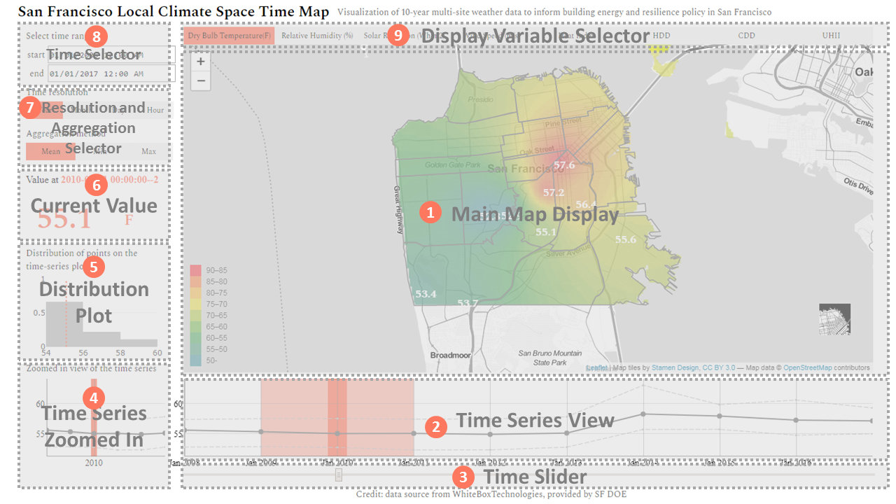
The interface has 9 major components, as is shown in the following figure

1. A main map display of a heat map of one of the raw (dry bulb temperature, relative humidity, solar radiation, and wind speed) or derived (heat index, heating degree day or HDD, cooling degree day or CDD, urban heat island index or UHII) weather variables
2. A time-series view showing the spatial-temporal aggregation (the solid line) and the spatial extremes (the min and max of the color-coded values displayed on the map, shown with two dashed lines) of the temporal aggregation of the selected variable
3. A time slider navigating through all time steps between the "start" and "end" dates specified in the time selector (component 8)
4. A zoomed in view of the time series plot within 3 time steps from the current time stamp
5. A distribution plot (histogram) of the spatial-temporal aggregation for the time range specified in the time selector, i.e. the distribution of the points on the solid line in the time-series view
6. A numeric display of the spatial-temporal aggregation at the current time step
7. A resolution and aggregation selector, specifying the temporal resolution of the display and how the weather station data is aggregated in the time dimension. For example, when the “year” resolution and the “mean” aggregation method are chosen, annual average data of each weather station (marked with white labels on the map) is computed and used to calculate a spatial interpolation of the whole San Francisco area for each year. The spatial average of values at all pixels on the map (for the chosen time resolution and aggregation method in component 7) are computed and displayed in the numeric display (component 6) and the time-series view (component 2) as points on the solid line. The spatial min and max of all the pixels on the map are displayed as points on the dashed lines in the time-series view. No aggregation method is available for the hourly data, as our source data is hourly. HDD and CDD only have three time resolutions (year, month, and day), because of the way they are defined
8. A time selector specifying the range of time period displayed in the time series view (component 2) and the end points of the time slider (component 3)
9. Weather variables for selection: dry bulb temperature, relative humidity, solar radiation, wind speed, heat index, HDD, CDD, UHII

Variable definition and how they are calculated

• Solar Radiation: it refers to the Global Horizontal Radiation in Wh/m2
• Heat Index: it is “a measure of how hot it really feels when relative humidity is factored in with the actual air temperature” (US Department of Commerce, 2018). The heat index calculation follows (NOAA/ National Weather Service, 2014)
• Heating Degree Day (HDD) and Cooling Degree Day (CDD): first a daily mean temperature (the average of the daily max and the daily min) is computed, if the daily mean is above some base temperature (50F in our calculation), then the difference between the daily mean and the base temperature is the cooling degree day for that day; if the daily mean is below the base temperature 65F, the difference between the daily mean and the base temperature is the heating degree day of that day. The heating or cooling degree day for a month or a year is just the total heating or cooling degree day for all days in that month or year
• Urban Heat Island Index (UHII): it is a modification of the UHII metric in (Dean, 2015). The following method is used to compute the urban heat island index of pixel p for duration \(\text{UHII}_{pD}\)

  $$\text{UHII}_{pD} = \sum_{h \in D} \mathbb{I}[\text{Urban(p)}] \cdot (\max(0, T_{ph} - \overline{T_{uh}}))$$

  where \(\mathbb{I}[\text{Urban}(p)]\) is an indicator of whether pixel p is of an urban land use type, and \(\overline{T_{uh}}\) is the average temperature of all un-urban pixels in San Francisco.

Introduction to the interface

The interface has 9 major components, as is shown in the following figure

1. A main map display of an energy consumption map of the variables (Total site energy, Electricity, Gas, Electricity demand)
2. A time-series view showing the spatial-temporal aggregation (the solid line) and the spatial extremes (the 25% and 75% quartiles of the color-coded values displayed on the map, shown with two dashed lines) of the temporal aggregation of the selected variable
3. A time slider navigating through all time steps between the “start” and “end” dates specified in the time selector (component 8)
4. A zoomed in view of the time series plot within 3 time steps from the current time stamp
5. A distribution plot (histogram) of the spatial-temporal aggregation for the time range specified in the time selector, i.e. the distribution of the points on the solid line in the time-series view
6. A numeric display of the spatial-temporal aggregation at the current time step
7. A time selector specifying the range of time period displayed in the time series view (component 2) and the end points of the time slider (component 3)
8. A resolution and aggregation selector to select the resolution and aggregation method for displaying energy data over time. This determines how the data is grouped and presented in the temporal dimension. The aggregation methods are summarized in the table below.
   
   

   Category	Unit	Aggregation method
   Total site energy	MJ	sum
   Electricity consumption	MJ	sum
   Gas consumption	MJ	sum
   Electricity demand	kW	min, mean, peak

   
   For instance, if the user selects a "month" resolution and the "mean" aggregation method, the average energy data for each month is calculated by considering all census tracks. These monthly averages are then used to generate a spatial interpolation for the entire Los Angeles area. In the selected resolution and aggregation method (specified in component 8), the numeric display (component 6) and the time-series view (component 2) represent the computed spatial averages of values from all census tracks as points on a solid line. In the time-series view, the dashed lines represent the 25th and 75th percentile values derived from the energy data of all census tracks on the map. These percentile values provide a visual representation of the distribution of energy data across the various locations within the map.
   N.B. Yearly and hourly data does not have an available aggregation method, as the source data spans one year and is provided on an hourly basis.
9. Variables to display: Total site energy, Electricity Consumption, Gas Consumption, Electricity demand

Introduction to the interface

The interface has 9 major components, as is shown in the following figure

1. A main map display of an anthropogenic heat emission map of the variables (Total heat emission, HVAC heat emission)
2. A time-series view showing the spatial-temporal aggregation (the solid line) and the spatial extremes (the 25% and 75% quartiles of the color-coded values displayed on the map, shown with two dashed lines) of the temporal aggregation of the selected variable
3. A time slider navigating through all time steps between the “start” and “end” dates specified in the time selector (component 8)
4. A zoomed in view of the time series plot within 3 time steps from the current time stamp
5. A distribution plot (histogram) of the spatial-temporal aggregation for the time range specified in the time selector, i.e. the distribution of the points on the solid line in the time-series view
6. A numeric display of the spatial-temporal aggregation at the current time step
7. A time selector specifying the range of time period displayed in the time series view (component 2) and the end points of the time slider (component 3)
8. A resolution and aggregation selector to select the resolution and aggregation method for displaying energy data over time. This determines how the data is grouped and presented in the temporal dimension. The aggregation methods are summarized in the table below.
   
   

   Category	Unit	Aggregation method
   Total Anthropogenic Heat Emission	MJ	min, mean, peak, sum
   HVAC Heat Emission	MJ	min, mean, peak, sum

   
   For instance, if the user chooses a "month" resolution and selects the "mean" aggregation method, the average anthropogenic heat data for each month is calculated by considering all census tracks. These monthly averages are then used to generate a spatial interpolation for the entire Los Angeles area. In the selected resolution and aggregation method (specified in component 8), the numeric display (component 6) and the time-series view (component 2) represent the computed spatial averages of values from all census tracks as points on a solid line. In the time-series view, the dashed lines represent the 25th and 75th percentile values derived from the heat emission data of all census tracks on the map. These percentile values provide a visual representation of the distribution of heat emission data across the various locations within the map.
   N.B. Yearly and hourly data does not have an available aggregation method, as the source data spans one year and is provided on an hourly basis.
9. Variables to display: Total heat emission, HVAC heat emission

References

1. CDC. (2017). Heat-related illness. https://www.cdc.gov/pictureofamerica/pdfs/Picture_of_America_Heat-Related_Illness.pdf
2. City of Fresno. (2020). City of Fresno Data Hub. https://gis-cityoffresno.hub.arcgis.com/
3. Four Twenty Seven. (2018). The California Heat Assessment Tool: Planning for the Health Impacts of Extreme Heat. http://427mt.com/wp-content/uploads/2018/08/427-CHAT-report.pdf
4. Hsiang, S., Kopp, R., Jina, A., Rising, J., Delgado, M., Mohan, S., Rasmussen, D. J., Muir-Wood, R., Wilson, P., Oppenheimer, M., Larsen, K., & Houser, T. (2017). Estimating economic damage from climate change in the United States. Science, 356(6345), 1362–1369. https://doi.org/10.1126/science.aal4369
5. U.S. Census Bureau. (2017). 2013-2017 American Community Survey 5-Year Estimates.
6. U.S. Census Bureau. (2018). American Community Survey and Puerto Rico Community Survey 2018 Subject Definitions.
7. Weather History & Data Archive. (2020, August). Weather Underground. https://www.wunderground.com/history
Time resolution
Aggregation method
Select time range
Start
End
Median value of the district at
A kW
Distribution of points on the time-series
Zoomed in view of the time series